

Platform · Model anatomy
Every layer, weight and bias, drawn and replayed.
The dashboard draws the structure you uploaded and walks a prediction through it in your browser, from the stored weights, with every step confirmed against the API's own trace. Here is one trace from the API reference, one operation at a time.
Model anatomy · a real trace
Follow one prediction through every weight.
A small churn network from the Kaimei API reference scores one customer. Scroll to walk the prediction through it one operation at a time, with every number written out as it is computed.
-
01 / 07The network
One network, one customer.
churn-net-docsis the example network in the API reference. All 27 of its parameters are uploaded, so every weight below is the one that computes the score. One customer waits at its inputs.Request body
{"input": {"tenure_months": 3, "monthly_spend": 91.5, "support_tickets": 4}}- 11 nodes
- 27 parameters
- 4 layers
- fidelity exact
-
02 / 07Standardise
Standardise each input.
The model stores a centre and a scale for every input. Three months sits 21 below the centre of 24; divided by the scale of 18, it becomes −1.167.
tenure_monthstenure(3−24)/18=−1.1667 monthly_spendspend(91.5−62)/30=0.9833 support_ticketstickets(4−1.2)/1.6=1.75The trace's own line
tenure months: (3 − 24) / 18 = -1.167. -
03 / 07Hidden layer
Four weighted sums.
Each hidden unit weighs the three standardised inputs and adds a bias. The edges carry the products: blue raises a unit, pink lowers it, thicker moves it more.
W·0.8−0.30.5 −0.60.90.2 0.10.4−0.7 0.3−0.20.9x+−1.16670.98331.75b=0.1−0.20.050h−0.25331.735−0.89831.0283h₁ = 0.8·(−1.1667) − 0.3·0.9833 + 0.5·1.75 + 0.1h₁ = −0.9333 − 0.295 + 0.875 + 0.1 = −0.2533
h₂ = −0.6·(−1.1667) + 0.9·0.9833 + 0.2·1.75 − 0.2h₂ = 0.7 + 0.885 + 0.35 − 0.2 = 1.735
h₃ = 0.1·(−1.1667) + 0.4·0.9833 − 0.7·1.75 + 0.05h₃ = −0.1167 + 0.3933 − 1.225 + 0.05 = −0.8983
h₄ = 0.3·(−1.1667) − 0.2·0.9833 + 0.9·1.75 + 0h₄ = −0.35 − 0.1967 + 1.575 + 0 = 1.0283
-
04 / 07ReLU
Two units switch off.
ReLU keeps positive values and turns negative ones into zero. Units 1 and 3 fall below zero for this customer, so their outgoing weights play no part in the score.
relu(−0.2533) =0unit 1 off relu(1.735) =1.735 relu(−0.8983) =0unit 3 off relu(1.0283) =1.0283What the trace hands the output
"input": [0.0, 1.735, 0.0, 1.0283] -
05 / 07Output
One logit, then a probability.
The output unit weighs the two live units and adds its bias of −0.3, giving 2.3927. The sigmoid maps that to 0.916, above the 0.5 threshold, so the label is churn.
z =
−1.2·0+ 0.9·1.735 +0.7·0+ 1.1·1.0283 − 0.3z = 1.5615 + 1.1312 − 0.3 = 2.3927
p = σ(2.3927) = 0.91626639
0.9163 ≥ 0.5 threshold churn
-
06 / 07Drivers
What moved the score.
The trace names the nodes that moved the final score, and by how much. The hidden layer pushed it up by 2.6927; the bias pulled it down by 0.3. By size, that is 90% and 10%.
fromdeltasharehidden__relu+2.69270.8998bias−0.30.1002Together
2.6927 − 0.3 = 2.3927 → σ → 0.91626639 -
07 / 07The API
The same walk, in one call.
The dashboard's anatomy view replays this walk in your browser, from the stored weights, with every step confirmed against the API's own trace.
trace = client.models.trace_structure(
    "churn-net-docs",
    input={"tenure_months": 3,
           "monthly_spend": 91.5,
           "support_tickets": 4})
print(trace.output)
# {'label': 'churn', 'probability': 0.9163, …}
Every number is from the churn-net-docs example in the Kaimei API reference (its spec, weights and trace response), for the reference's example customer. Values the reference elides with “…” are recomputed from the same weights, and every value it does print matches. Products are rounded to four decimals; sums use full precision. The drawing and its timing are made for this page; the dashboard draws the same structure in its own anatomy view.
Model anatomy · titanic-forest
Walk a real forest, one passenger at a time.
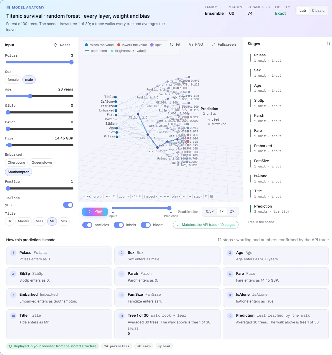
The random forest from the Titanic example, drawn the way the dashboard draws it: ten inputs, one of its thirty trees, and the prediction. Change the passenger and the path moves. Every number is worked out in your browser from the model's own splits and leaves.
Model anatomy
Titanic survival · random forest
Forest of 30 trees. The scene draws tree 1 of 30; a trace walks every tree and averages the leaves.
- Family
- Ensemble
- Trees
- 30
- Nodes
- 1,430
- Fidelity
- Exact
FamSize 2 · IsAlone no
from SibSp + Parch + 1
Replayed in your browserfrom the forest's 1,430 nodes. For all 891 passengers in the training file it gives the same P(survived) as scikit-learn, and Mr Braund's 7.4% is the figure the API returns in notebook 01.
In the dashboard
The same walk, for any model you upload.
- Trees, forests, linear models and MLPsDrawn node by node, with the path a prediction takes highlighted.
- Keras and PyTorch networksLayer graphs including convolutions, pooling, residual adds and concatenations.
- Large models stay readableRepeated blocks fold into one, so encoder.layers.0 to 47 becomes a single ×48 block, and tensors load only when you open them.
Upload a model this afternoon.
The free plan covers the whole Titanic walkthrough with room to spare. Your own model is one call away.